MMG Medical Tools
Bloch Simulator
The Bloch Simulator serves for
- Creation of MOLLI sequences database by simulating the MRI scanner based on different T1 relaxation time. The user may set-up different parameters of the virtual scanner.
- Use the database for more accurate evaluation of T1 maps.
Using the Bloch simulator to get T1 map
Command-line interface (in Linux)
Enter the directory with the DICOM data. Call bloch-simulator-read-dicom application as
bloch-simulator-read-dicom .
It will extract necessary data from the acquisition to a file SetupFile.txt and DicomData.txt. After that, execute the bloch-simulator-create-database application as
bloch-simulator-create-database --directory .
which creates a file Database.txt. This program is simulating MOLLI sequences using the Bloch equations. It creates database for large number of different setup parameters. One of them is the size of initial vector of magnetization M=(0,0,M0). M0 changes from --startM0 (0.05 by default) to --endM0 (1 by default). It grows by 0.025 in each step. It usually has no sense to make these parameters larger than 1. Another important parameters in the Bloch equations are T1 and T2 times in ms. T1 changes from --startT1 (200 by default) to --endT1 (1200 by default) and it grows by 1. Similarly T2 changes from --startT2 (40 by default) to --endT2 (50 by default) and it grows by 5. In fact, the simulator does not simulate relaxation of only one spin but rather of group of spins referred as isochromat. During the simulation, several RF pulses are applied to tilt the magnetization vectors of the isochromat. Each vector is tilted a bit differently which we approximate by the Gaussian distribution with zero mean and prescribed variance. This variance changes from --startVariance (40 by default) to --endVariance (60 by default) and grows by 10. Finally, the Bloch simulator simulates the off-resonance effect which is a difference between the Larmour frequency of a spin isochromat and the excitation RF pulse. It is given in Mhz and changes from --startOffresonance (50 by default) to --endOffresonance (70 by default) and it grows by 10. The last parameter is --sequence (3-3-5 by default) which serves for choosing either 3-3-5 MOLLI sequence or 5-5-3 MOLLI sequence.
In the last step, we will use the precomputed database for T1 map reconstruction from the measured DICOM data. Run the program bloch-simulator-create-t1-map as
bloch-simulator-create-t1-map --directory .
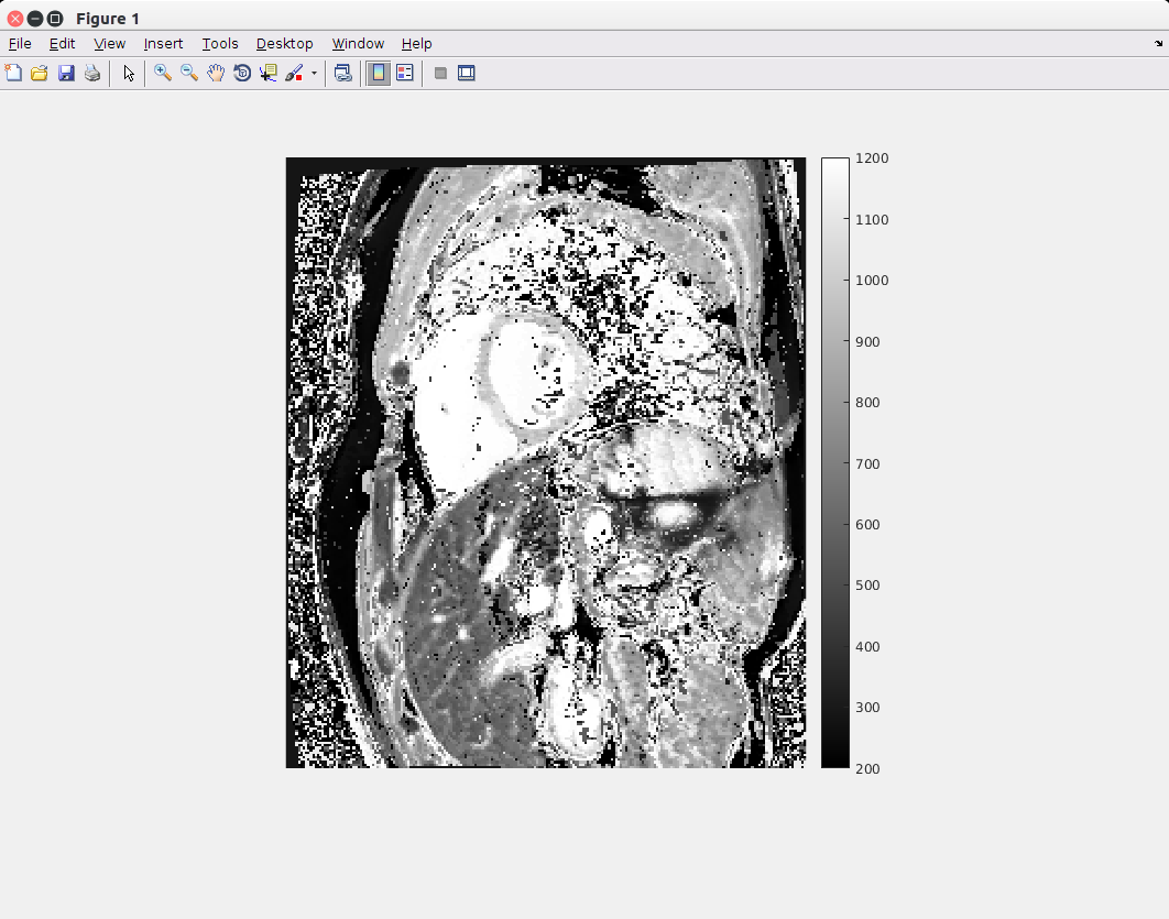
The program creates files with T1 and T2 maps called T1map.txt and T2map.txt. You may open them in Matlab by clicking on a button Import data, choosing the file with the map and Numeric Matrix as a type of imported variable. Then click the green check button to import the data. Finally you may visualize the map by a MATLAB command
imshow( T1map , 'DisplayRange', [])
in case of T1 map. You should get a result similar to the following.
Graphical user interface (Linux and Windows)
Calling the previous three programs without command-line arguments invokes their graphical interface.
Read DICOM GUI
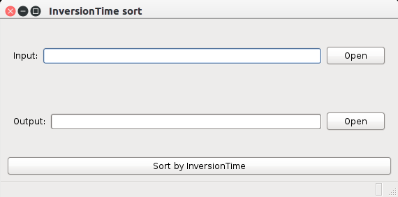
Just select input and output directory and press the button. The program will recursively process even all subdirectories.
Create database GUI
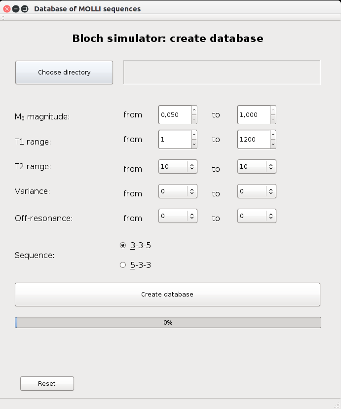
You first need to chose a directory with the data you want to process. This directory needs to contain the file SetupFile.txt. The next buttons serves for setup the parameters intervals. Meaning of all parameters is described in section about the command-line parameters.
Create T1 map GUI
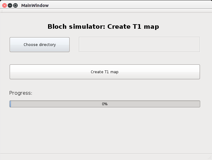
Just choose the directory you want to process and press the button „Create T1 map“.